
INU01 /1 - System Setup Constants, Defaults and Rules
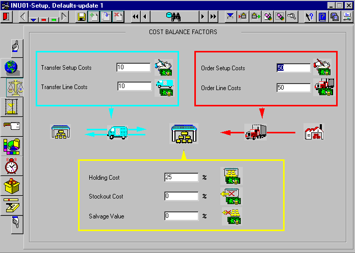
INU01 /2 - Cost Balance Factors
INU01 /4 - Order and Transfer Constraints
INU01 /5 - Safety Stock Modulation Matrix
INU01 /6 - Order Time Statistics
INU01 /7 - Consumption Statistics
INU03 /2 - Item Control Parameters
INU04 /1 - Stock Administration
INU09 - Control Centers, Managers
MAU01 /2 - Forecasting Methods
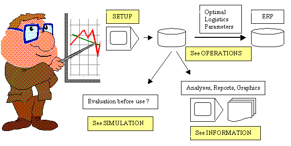
When the general stores configuration, supply and distribution networks have been defined, the majority of the logistical reorder problems can be solved automatically by means of computer programs, which use generally available statistical information. This information consists of dynamical data, such as issues and purchasing transactions, basic item and classification data, stores constants, and tuning factors for which an optimal value can be defined and which modify the working of the programs.
The purpose of this manual is to provide information about the system definition and setup. Only after complete setup, operations support can be given and programs, analysis and reports can be run.
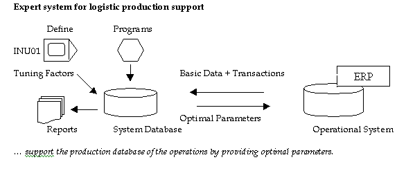
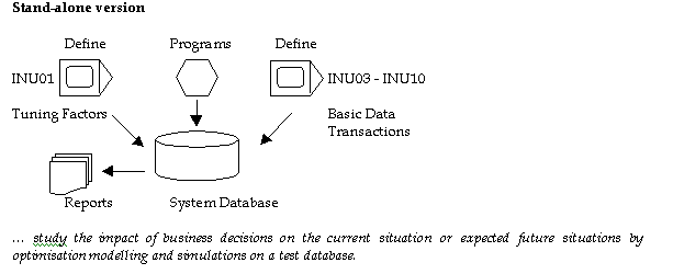
The system can be setup as expert system for logistic operations support of the current real life situation on the production database, or to study the impact of business decisions on the current or expected future situations, by optimisation modelling and simulations on a test database.
This manual describes the functions related to basic data and tuning. Basic data consists of those data that may be regarded as elementary data whereas dynamic data is created by business events and depends on the elementary data. The system contains a complete set of basis functions and database tables (its own house holding).
Normally transactions will originate from business events of the production, or they can be generated by simulation. The function INU08 allows transactions of business events to be entered for simulation and modelling.
The following functions define the setup, the basic data and tuning.
INU02 - Parameter groups
INU03 - Items definitions
INU04 - Stock data
INU05 - Stores and Network
INU06 - Suppliers
INU07 - Clients
INU08 - Transactions
INU09 - Control Centers
INU10 - Locations
MAU01 - Forecast Methods, Tables and Weighting Schemes
The operations support functions (see OPERATIONS manual)
INU12 - Exceptions handler
NOTE: The function ordering presents also the order in which data should
be defined, to get the system operational. e.g. First general constants
and rules in INU01, then control parameter group definitions INU02, then
items in INU03, which may be linked to a parameter group defined in INU02.
The basic data can be entered and modified in screens and consist of mandatory data and non-mandatory details. For INU01 recommended defaults values are provided, which normally do not need to be adjusted. After tuning most of the set-up functions do not need any manual attention anymore. In stand-alone version or for simulation and modelling study purposes the functions INU03 - INU10 can be used to enter or change the basic data manually.
In production situation where the system is used as expert system to support another operational ERP (Enterprise Resource Planning) system like SAP, BAAN, ORACLE Logistics, the information in INU03 - INU10 is normally automatically maintained by interface to the operational ERP system. Only INU12 should be used during production, to support manual exceptions handling.
SETUP INU01
Only at setup. Recommended defaults are provided.
INTERFACE INU03 - INU10
Data automatically maintained by interface to production.
MANUAL INU02, INU11, INU12
Manual, to enter constraints and to handle exceptions.
PARAMETER GROUPS
A number of management input, steering or control parameters are needed in the logistical calculations, such as target service-level, holding cost, fixed and variable order costs, absence cost, item review and entry time. Although DEFAULT values can be defined in the setup function INU01, which will serve most of the items, groups of items may still exist which should be treaded differently. e.g. They may have a higher order line cost, or a longer review time caused by a required inspection, or management may want to set a higher target service level.
For these groups of items it is not necessary to define the control parameters for each individual item. It is sufficient to enter the NOT-DEFAULT control parameters on a single parameter group record in INU02 and link this control parameter group record to the group of items in INU03.
In this way maintenance work is decreased and control is increased in a simple and easy way.
Only if an item needs its own UNIQUE control parameters, these control parameters should be defined for this item in INU03 /2.
The values of the control parameters can thus be specified on a number of levels. These levels define a hierarchy, which is followed when the value of a parameter is retrieved for use in a calculation.
HIERARCHY Item - Parameter Group - Default
If a constant is defined on item level, this value is taken, if it is not defined on item level, the value defined to the control parameter group is used, if this value is not defined, the overall default value defined in screen INU01 is used.
NOTE: Never enter a 0 if you want to leave a parameter undefined, the 0 will be taken as a value, only an empty, blank field denotes an undefined parameter.
If one only wants to use global values, define the default parameters
in screen INU01 only: overall service level, holding cost, fixed and variable
order costs, absence cost, review and entry time. All calculations will
use these values. Definition hierarchies for the different parameters:
|
||||||||||||||||||||||||||||||||||||||
|
|
||||||||||||||||||||||||||||||||||||||
|
||||||||||||||||||||||||||||||||||||||
NOTE: As defaults for the item control parameter are NOT hard-copied into item records, but dynamically determined at calculation time, just a view high level parameters, whose values may be changed at any time, may control all the items.
The user sets the objectives and targets in INU01. Occasionally occuring non standard situations can be handled by defining additional parameter groups in INU02.
SIMULATION
Simulate by "real history replay method" (using real historical data with different calculated parameter sets) the impact of business decisions, analyse simulation results, trace exceptions, use optimisation modelling techniques to find optimal parameters and business policies
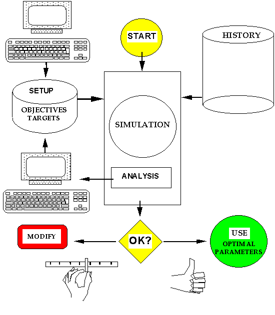
A number of target or control parameters highly influence the results of the logistic calculations, some of these parameters must be defined (service level, holding cost, order cost, review time) while others are derived by statistics (demand statistics, lead times).
E.g. the economical order quantity EOQ depends on the total order cost and holding cost, the item cost price, stock demand or item consumption, and out of stock costs. The safety and buffer stock depends on the lead time and customer order statistics and requested service levels.
Service Level
Service level in percent %
100x (Number of successfully served requests/Total number of requests)
Holding Cost
Cost of holding the item in stock, calculated as percentage of the average
value in cost price of the items hold in stock, by year.
An often by management imposed constraint is that the total stock value
should not exceed a certain defined amount: the investment limit.
Fixed Order Cost
Fixed part of order or administrative cost. Cost of processing the order
through accounting and invoicing, including order system costs.
Variable Order Cost
Variable part of order or order-line cost, involves handling, transport
and insurance, it may include manufacturing costs of the product for various
order sizes, distribution, inspection and entry.
Absence cost
Percentage, which is used to calculate the loss of profit to sales, when
the item is not available to sales.
If the gross profit is defined by Qty * (Sales price- Cost price)
then Loss = BO Qty x Profit x (Absence cost/100)
An estimate of the yearly loss can be given as (1-Service Level/100) x
Year turnover Qty x Profit x (Absence cost/100)
To sales it is important how much you are selling or not selling because
the item is not available and the loss resulting from it. Absence cost
is useful to calculate the cost of lost sales.
e.g. If a customer has to wait, for his order to be filled, the loss or
absence cost is 0 %, if the customer does not wait and the customer order
is lost to a competitor the absence cost is 100 %, if the customer is
a regular client, but does not order anymore if an order can not be filled
the absence cost or loss to sales may be higher then 100 %
Stock-out Cost
Expected real cost caused by stock-out per order cycle. This cost is of
another type then the absence cost (see Operations Manual), and is more
related to costs which occur when an item, cannot be issued for planned
production or repair. The costs of lost production and costs of changing
the work plan, and rescheduling the operations can be considerable. This
cost is calculated per unit of the item.
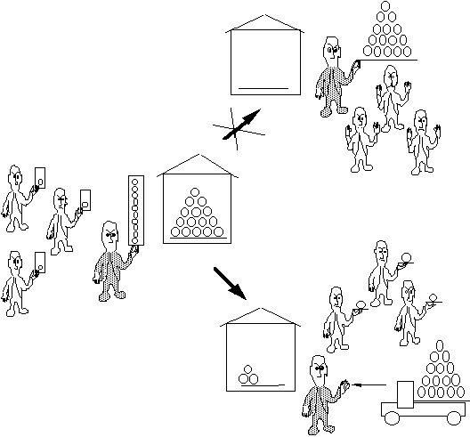
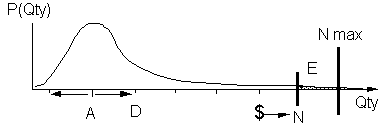
Exception threshold
Exceptional large non-recurrent, or infrequent occurring large demanded
quantities will lead to stock-outs and unsatisfied normal customer orders
(see picture). If these exceptional large demands must equally well be
satisfied from stock, this will lead to non-economical extremely high
safety stock situations. To avoid these unwanted situations the demanded
quantity is checked against the exception threshold level or break
quantity. If the demanded quantity is above the exception threshold
level, it is turned into a special order or so-called Direct Out.
Demanded quantities below the exception threshold level are considered
to be Normal Demand, and are normally served from stock.
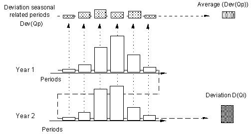
Pattern Factor A system seasonal pattern flag is set, if the average
deviation of the consumption over seasonal corresponding periods divided
by the average deviation over all the periods is smaller then a threshold
defined in the setup function INU01.
Avg (Dev (P Seasonal)) / Dev (P) compensated for trend, calculated over
a minimum of 2 years.
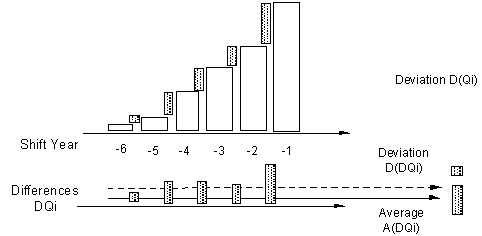
Trend Years A system trend pattern flag is set, if over the last years there existed a steady increase or decrease: the trend gradient value was large, with a small variation of this gradient.
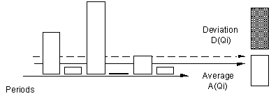
Lumpiness Factor A lumpy demand system flag is set if the normal
stock demand Q calculated by month is very variable, as defined by the
ratio of the deviation to the average demand sampled in month periods.
Dev (P) / Avg (P) > in setup INU01 defined factor.
The lumpy or erratic demand may be perpetual, composed of periods of little
or no demand followed by periods of high demand.
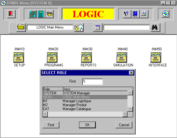
In order to access the setup and basic data functions one has to select the role LOGIC main menu
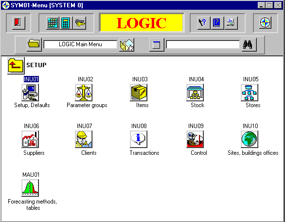
INU01 /1 -SYSTEM SETUP CONSTANTS, DEFAULTS AND RULES
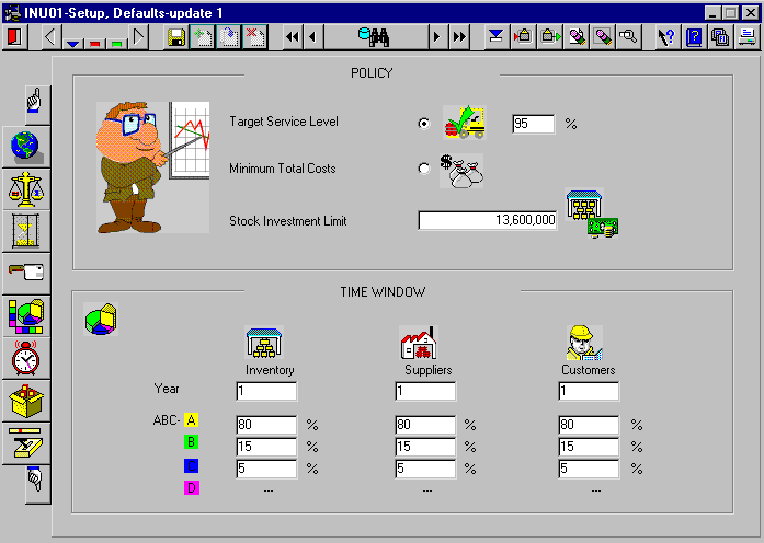
FUNCTION AIM
The purpose of this function is to define general system settings, it allows to define DEFAULTS for the target or control parameters. Such as target service level, holding cost, fixed and variable order cost, stock-out cost, time windows, management objectives, rules and constraints.
FIELDS
Target One can define an overall target service level or one can choose for the minimisation of the total cost, in the case of minimum total cost, the service level for each item is a result of the minimum total cost calculation.
Investment Limit This constraint sets a limit to the total average amount in item cost price, of inventory that may be carried by the stores.
Time Window A summary of historical events like number of orders, total quantity and amount, for a time window or period of history is kept on the inventory item, supplier and customer records and used as input to the ABC analysis. Different time windows and ABC threshold percentages can be defined.
HOW TO USE THE FUNCTION
Set the parameters to the desired values. By pressing <TAB> buttons on the left one can reach other tab pages. Not all fields are mandatory.
INU01 /2 - COST BALANCE FACTORS
DESCRIPTION
The purpose of this screen is to define the general cost balance factors. In general there is a cost to order/transfer an item, which is composed of 2 components: the order/transfer setup cost and the order/transfer line cost for each additional item. It costs to have or possess the item, the so-called holding cost. It may also cost if an item is not directly available from stock when there is a material request for this item, the so-called stock out cost. Finally there is a certain cost related factor if the item is hold in stock but there is no demand for this item.
FIELDS
Order/Transfer Setup cost Fixed part or administrative part
of the order or transfer cost.
Order/Transfer Line cost Additional cost for each order line
or transfer line.
The total Order/Transfer cost can be defined as order setup cost + line cost x number of lines.
Holding cost Cost of possession as percentage of the average
item value per year.
Stock out cost Extra cost if the item is not issued on demand.
Salvage value If there is no demand for an item, it still may have
a certain salvage value, which represents the reclaimable value, which
may be recovered if the item is returned to the supplier or sold out under
discount.
DESCRIPTION
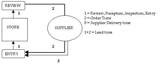
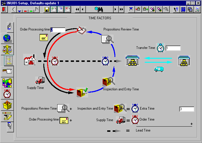
The purpose of this screen is to define the general time factors. Some time factors can be obtained from the system history, like time between ordering and reception, while other time factors have to be estimated and entered by the user, like administrative time of reviewing the re-order propositions, inspection and entry of received ordered items into stock.
FIELDS
Order time
Time elapsed between the order sending and reception of the ordered material.
Extra time
Estimate sum of all the administrative components that have to be added
to the order time, like re-order propositions review time, reception and
inspection time, time to enter the item in stock.
Lead time
The total time elapsed in the reorder process between the moment a replenishment
need is detected and an order proposal is generated, and the availability
of the item in stock to sales of the re-ordered item.
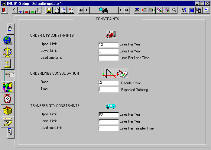
The purpose of this screen is to define general order and transfer constraints. These constraints are logical and generally defined by the management to avoid unwanted situations. e.g. It may be economical to order 3 years of material, but management wants to stock not more then 0.5 year of expected consumption: a lower order frequency limit constraint of 2 will restrict the EOQ quantity of 3 years (frequency 0.33 lines per year) to 0.5 year of expected consumption.
ORDER/TRANSFER CONSTRAINTS
Upper limit Limits the number of orders per year, or inversely poses a lower limit to order quantities as compared with the expected year consumption.
Lower limit Lower order frequency limit. This condition poses an upper limit to the quantity ordered per year.
Lead time limit A long lead time and small economical order quantity EOQ may lead to multiple orders in the lead time. This constraint limits the number of orders that may simultaneously exist. It relates the order quantity to the consumption in the lead time, imposing long lead times to result in a larger order quantities.
CONSOLIDATION
Ratio ROP Ratio of the pull down quantity and the reorder point
Time Days of daily consumption before reordering
CONSOLIDATION
The consolidation process aims to synchronise ordering of items for the same supplier and contract, and results in orders with many order lines. It works by pulling other items into reordering condition, when one item is normally to be reordered for a given supplier and contract. In order to get other items into reordering the reorder points are artificially increased.
A number of factors can be defined.
If more factors are defined they will work together: if one condition is not met, but another is satisfied, the item will be pulled down into reordering. The consolidation process is stopped after the following conditions are reached
Minimum value for the order is reached
Maximum number of order lines for the order is reached.
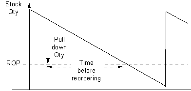
A number of limits to the increase of reorder point can be defined, each limit having its own benefits.
Ratio ROP (OH-ROP) / ROP < limiting condition
The increase limit by ratio of the pull down quantity = (quantity in stock OH - quantity reorder point ROP) and the reorder point. This condition has the disadvantage that there is no control on the extra costs.
Time (OH-ROP)/Daily Consumption < limiting condition
The increase limit by the pull down time = (quantity in stock OH - quantity reorder point ROP) / Daily Average Consumption. This has the advantage that items that will soon normally come into re-ordering, are re-ordered grouped together.
INU01 /5 - SAFETY STOCK MODULATION MATRIX
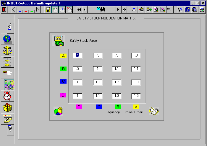
DESCRIPTION
The safety stock quantity is calculated as a function of the service
level and item demand history.
Factors in this calculation are variability in expected demand quantity
and number of demands and lead time, but there are NO economical cost
price conditions imposed.
This matrix allows modulation of the safety stock quantities by multipliers
in an economical way, by obtaining higher service levels at relatively
low extra holding costs. If the factors are taken larger then 1, the safety
stock quantities will be larger, and higher service levels, then set by
the target service level definition will be obtained.
The matrix horizontal axis represents the ABC classification by frequency
or number of demands
The matrix vertical axis represents the ABC classification by safety
stock value
MATRIX FIELDS
|
|
|
|
|
|
|
|
|
|
|
|
|
|
|
|
|
|
|
|
Coefficient AA - (item demand ABC = A, safety stock value ABC = A)
Coefficient AB - (item demand ABC = A, safety stock value ABC = B)
INU01 /6 - Order Time Statistics
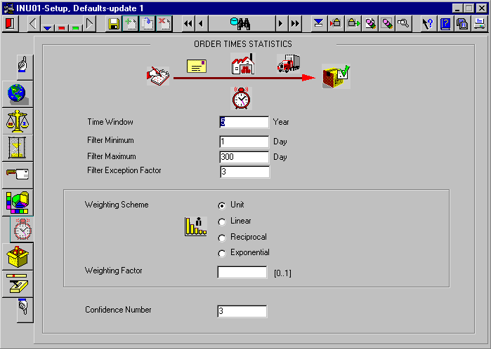
DESCRIPTION
The purpose of this screen is to define or change order time statistics
calculation factors.
The parameters defined in this function will be used to calculate order
delays for suppliers and supplied items.
FIELDS
| Time Window | Time window in years of transaction history used. |
| Filter Minimum | Order delays below this number will not be used in the calculation. |
| Filter Maximum | Order delays above this number will not be used in the calculation. |
| Filter Exception Factor | Data larger then the average order time times this factor will not be used in the calculation. |
| Weighting scheme | Weighting scheme used, to calculate the average order time and deviation. |
| Weighting factor | Smoothing factor used in the weighting scheme to give more weight to recent transactions |
| Confidence number | Below this number, there are insufficient transactions for the item, and a combination of supplier and item statistics is used. |
DATA ERRORS and ACCURACY
New order delays are calculated based on order transactions. From these transactions the average and deviation are calculated. However, the results of this calculation are highly sensitive to data errors, abnormalities, and historical time interval used. Different filters can be defined to avoid abnormalities and enhance the accuracy of the statistics.
FILTERS
Time window historical data
This filter limits the historical transactions used to a pre-defined number
of years
e.g. historical data > last 5 years
Fools filter
The fools filter or data entry errors filter, filters the logical abnormalities
out
e.g. order delays > 365 days and order delays < 0 due to data entry
errors are filtered out
Statistical exceptions filter
The statistical exceptions filter, filters the statistical abnormal events
out for order delays > Factor x statistical average.
e.g. order delays > 4 x statistical average
STATISTICS
After filtering the data, the order time statistics is calculated
Deviation order time D = Sqrt ( Sum ( (L -A) 2 ) / N(L) )
Therefore historical time dependent weighting, based on the number of years should increase the accuracy
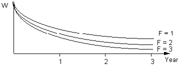
Weighting schemes S and weight formula W
D = Sqrt (Sum (W x (L -A) 2) / Sum (W))
Unit: W=1, No weighting
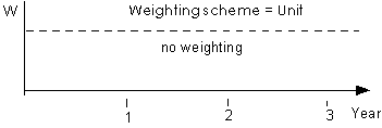
Linear: W = greatest ((Factor-Y), 0)
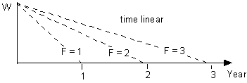
Reciprocal: W = 1/(1+greatest ((Factor xY), 0))

Reciprocal: W = exp (- Factor xY)
CONFIDENCE
In case of item introduction or change of supplier there are often insufficient data to determine accurate order times statistics by item with confidence. Therefore the algorithm calculates in 2 steps.
2. order time statistics by item.
D (Item) = beta x D (Supplier) + (1- beta) x D (Item)
Note: at T=1 D (Item) by definition = 0 and D (Item) is taken as D (Supplier)
INU01 /7 - Consumption Statistics
DESCRIPTION
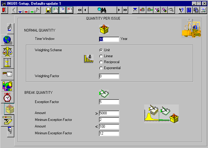
The purpose of this screen is to define single demands statistics factors like average expected quantity per demand and exceptional threshold level or break quantity formula factors.
FIELDS
| Time Window | Time window in years of transaction history used. |
| Weighting scheme and factor | Single demanded statistics may be calculated using time weighting. Weighting focuses the calculation on more recent issues. |
| Exception Factor | The exception factor N determines the statistical exception threshold
level or break quantity E = A + N x greatest (A, D). The exception level may be constraint by economical factors. |
| Maximal Value Constraint | If the value of the exception > maximal value, the factor N is shifted to a smaller value, this smaller value however has a lower limit, defined by the minimum factor. |
| Minimal Factor | Minimum value N may take under Maximal Value Constraint. |
| Minimal Value Constraint | If the value of the exception < minimum value, the factor N is shifted to a larger value, this larger value is restricted by the maximum factor, imposing the upper limit. |
| Maximal Factor | Maximum value N may take under Minimal Value Constraint. |
EXCEPTIONS
The exceptional threshold level or break quantity is defined to avoid
stock-outs, which will be caused by serving non-recurrent or infrequent
occurring exceptional large demands from stock. If infrequent occurring
exceptional large demands are included into the statistical demand used
to calculate stock replenishment parameters, this also will lead to high
safety stock values.
Careful definition of an exceptional threshold level quantity, above which
a demanded quantity will be served by a special order or direct-out, instead
of being served from stock, will lead to high service levels in combination
with low stock values.
A definition of statistical infrequent large demands can be formulated
by the demand statistics parameters average and deviation. Requests for
a quantity E larger then the average A plus N standard
deviations D will occur only with very low probability.
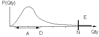
Sometimes D is very small or even zero e.g. when for a large number of demands always the same quantity is requested, thus a more practical definition is given by
E > A + N x greatest (A, D).
The above definition, does not include any price considerations. Practically
one wants expensive items to be served by direct-out quicker (less rare
in statistical sense) then very cheap items.
Economical conditions can be imposed by shifting N to a smaller
value (less rare occurrence of exceptional demand) if the cost of the
break quantity E is very large.
This constraint will lead to quicker ordering by direct-out of expensive
demands.
To avoid a very small value of N, a minimum can be defined in INU01
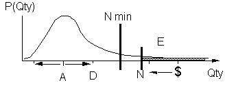
The same reasoning like above, but now for cheap items, leads to shifting the N to a larger value if the cost corresponding to E is very small. This constraint leads to nearly always serving from stock of cheap item demands even if they very seldom occur. To avoid a very large value of N a maximum can be defined.
If there is sufficient quantityin stock, an exceptional large
demand may be served in the normal way from stock.
This is the case if after serving at least one reorder point + average
daily consumption is left.
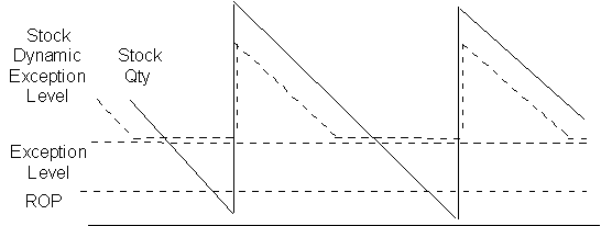
In order to avoid manual checking this condition for all daily exceptions, a so-called stock dynamical exception threshold level can be calculated such that after serving the exceptional demand at least
(Stock Dynamic Factor) x (the reorder point + daily consumption)
should be left in stock for normal serving and reordering
NOTE 1: The stock dynamic break quantity, is dependent on the situation of the stock, therefore it should be daily recalculated.
NOTE 2: The statistical quantity used for forecasting of normal demand depends on the statistical exception level, or user defined as constraint direct-out level but NOT on the stock dynamical level.
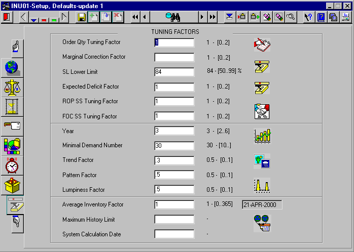
DESCRIPTION
The purpose of this screen is to set or modify a number of factors, which influence the logistics in a global way. For instance all economic order quantities are multiplied with a tuning factor, whose value is normally set to 1, assigning any other value will increase or decrease all order quantities. In this way the user can control and globally fine-tune the logistics to his own judgement, for instance set all order quantities to a global larger or smaller value.
FIELDS
| Order Qty Tuning Factor | Globally modifies the economical order quantities. The order stock
quantity is multiplied with the Order Qty Tuning Factor NOTE: This factor is applied BEFORE the order constraints (see INU01/4) are applied. |
| Marginal Correction Factor | This term is important for items which are perishable (e.g. ink) or have a short and defined shelf life, or the demand for them is a one-time event (e.g. agendas). As the demand is variable and covered by a single order (e.g. when the expected consumption in the shelf life < EOQ) there may be a loss calculated by the salvage value for unsold product, as well as a lost profit if the demand exceeds the ordered quantity. The order quantity that will maximise profit can be calculated from the expected demand plus a correction depending on the deviation of the demand, the cost price, the sales price and the salvage value. This correction is multiplied with the Marginal Correction Factor. |
| SL Lower limit | Target service level is defined over the total time the item is served from stock. This time consists of two parts: The time in which the stock above the reorder point quantity will be consumed, and the time during which reordering takes place. If the first component is relatively large, this may by definition lead to a low service level to be satisfied during the lead time. To ensure that also in the lead time there is sufficient service, a minimum service level can be defined here. |
LOWER LIMIT
The service level for an item is defined as the ratio of the number of requests that can be immediately satisfied from stock and the total number of requests.
Service Level in % = 100 x Number of served requests/ Total number of requests for material
The target service level is defined over the total time the item is kept in stock. Normally there is only a possibility on stock-out and backorders after the quantity in stock has reached the reorder point. For the time the stock is above the reorder point, almost 100 % service level is ensured.
If the order serve time is very large compared with the reorder time, this will by definition lead to a low service level in the lead time, to reach the overall defined target service level.
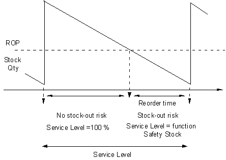
Because the on-hand quantity can drop significantly below the re-order point by the triggering demand, when the re-order proposal is created we may adjust the ROP to compensate for it. That is, in addition to the demand in the lead time plus the safety stock that usually make up the ROP, we now add the expected deficit term to the ROP, which is the average amount that the quantity on hand is likely to fall below the reorder point when triggering the re-order proposition. To switch off and on, and to fine tune this term is added multiplied with the Expected Deficit Factor.
ROP SS Tuning Factor
This term is important if one globally wants to modify the calculated
safety stock quantities. The safety stock quantity is multiplied with
the ROP SS Tuning Factor.
This factor is directly applied to the safety stock component
FOC SS tuning factor Allows to fine tune the FOC safety stock in maximum or fill-up-to level. This factor is directly applied to the safety stock component
For a number of years and a minimum number of demands in
these years the trend, pattern and lumpiness are derived and corresponding
flags are set on the stock item (see INU04 /2)
See DEFINITIONS - the sensitivity of calculation can be increased or decreased
by the
Trend Factor, Pattern Factor, Lumpiness Factor, set stock
item Flag or Sign if
Sign (dQ) equal, dQ/Q > Trend Factor
Dev (Qs) / Dev (Q) < Pattern Factor
Dev (Q) / Avg (Q) > Lumpiness Factor
Average Inventory Factor Normally the quantity in stock fluctuates
very much as result of the replenishment cycles, and the average quantity
kept in stock is important management information, it is very convenient
to keep a time weighted exponential smoothed average of the qty in stock
S(Q) on the stock record for reporting purposes:
t = system time - last calculation date
f = t / ( t + 365 x ASF)
S (Q) = f x Q + (1-f) x S(Q)
NOTE: The calculation is somewhat insensitive to the period between re-calculations. The algorithm can be re-run on the same day (no action), or re-run in intervals of days, weeks or every month and still results in about same smoothing which depends on the factor ASF but not on the period between different runs.
Maximum History Limit For data maintenance, when defined, older history will be removed
System Calculation Date If this field is defined its value is used in the calculations instead of the SYSTEM DATE. It should normally NOT be defined.
FUNCTION AIM
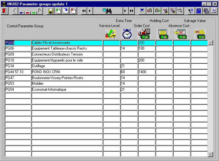
The purpose of this screen is to define parameters groups. The parameters target service level, cost of holding, order line cost, cost of absence can be specified. If the parameters are not defined on the item level (INU03) and a parameter group is associated with the item, the parameters of the parameter group will be taken instead of the defaults (INU01).
FIELDS
Code, Description Unique identification
code, description of the parameter group
Service-level, Extra time, Cost of order, Cost of holding, Cost of
absence, Salvage value
See HIERARCHY and DEFINITIONS
HOW TO USE THE FUNCTION
Enter the code and group description. The parameters do not need all to be defined, if the item specific or default values are to be used for the item. When pressing <DELETE RECORD> a warning will be used when the group code is in use, the group code will be removed from the items using the class when <COMMIT> is pressed.
FUNCTION AIM
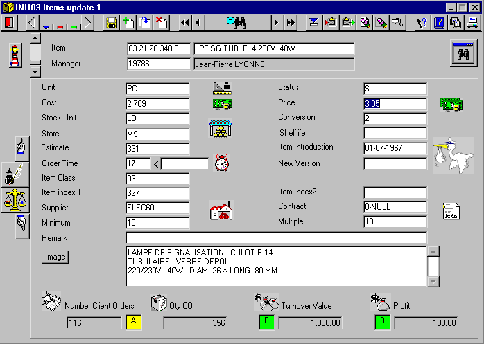
The purpose of this screen is to define or modify item definition and classification details.
FIELDS
| Item code, Description | Unique identification code, item description. | |
| Control | Item responsibility center/party or person, Manager | |
| Unit | Unit of Measure UM, Basic Unit - this is the accounting unit. | |
| Status | Identifies events in the life cycle. E.g. new/ active / not active. | |
| Cost | Average unit cost: this cost is used to evaluate the stock value and calculate the economic order quantity. | |
| Price | Sales price, which is charged when the item is sold. | |
| Stock Unit | Default stocking unit | |
| Conversion | Conversion factor between UM and stocking unit | |
| Principal Store | Main store, which is replenished for the item in a single re-order point many stores configuration. Purchasing is only re-ordering the item for this store, this store however may feed many satellite stores by inter warehouse transfer | |
| Shelf-life | The number of days the item can be held in stock before it will not be fit for consumption anymore, e.g. it will deteriorate or corrode after this date. | |
| Estimate | Initial year consumption quantity estimate for a new item. On introduction of a new item, there is no statistical data, the year estimate will be used to calculate the initial parameters. | |
| Introduction | Introduction /creation /item definition data. | |
| Order time | Time needed for the supplier to deliver the item. | |
| New Version | Date on which a new version of the item is due. | |
| Class | Identifies the physical class | |
| Index 1 | Free user definable index 1 e.g. Type identifies the logical class or use as spare part or consumable or cleaning use. |
|
| Index 2 | Free user definable index 2 | |
| Principal Supplier | Supplier at which the item normally will be reordered. Lead times statistics are calculated and the contract is valid for this supplier. | |
| Contract | Current valid contract. | |
| Order Minimum | Minimum order quantity. This is an order condition imposed by the principal supplier. | |
| Order Multiple | Incremental or order multiple quantity. This is an order condition imposed by the principal supplier. | |
| Remark | Free user definable remark or text. The <LIST VALUES> button will display a list of remarks for the current item control responsible or manager, for retrieving (enter query or interrogation mode) or definition. | |
| <IMAGE> | When pressed the item image is displayed (see INU04 /1) | |
| Description | Item text |
HOW TO USE THE FUNCTION
Use <CREATE RECORD> to enter an item. Item properties can be selected
using help screens by pressing <LISTVAL> on the item class field.
By pressing <TAB> on the left of the screen, the next TAB page will
display a number of target or control parameters which are used by the
logistical calculations.
INU03 /2 - Item Control Parameters
DESCRIPTION
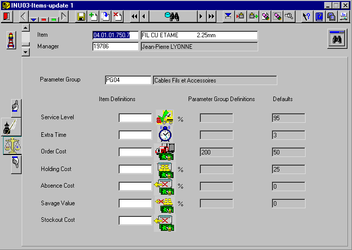
This page allows to link a parameter group to the item, and/or to define specific values for the target or steering parameters to the item. When a parameter group is defined for the item its target parameters are shown. The DEFAULT values defined in INU01 are shown as well.
FIELDS
| Parameter Group | A parameter group can be linked to the item, providing specific control parameters specific to the item. |
| Service Level, Order Cost, Holding Cost, Absence Cost, Salvage Value | see Definitions |
| Extra time | Review/Entry time: Total time needed to review and confirm, and to enter in stock of the ordered item. This time may include the extra time needed for assemblage or inspection, before the item becomes available. |
| Stock-out Cost | Estimated cost of stock-out, usually related to costs which occur when a planned item, cannot be issued, or cost of production stop if the item is used as spare part. Costs of changing the work-plan, and re-scheduling the operations, or production failure can be considerable. NOTE: This cost is defined per unit of the item. |
INU04 /1 - Stock Administration
FUNCTION AIM
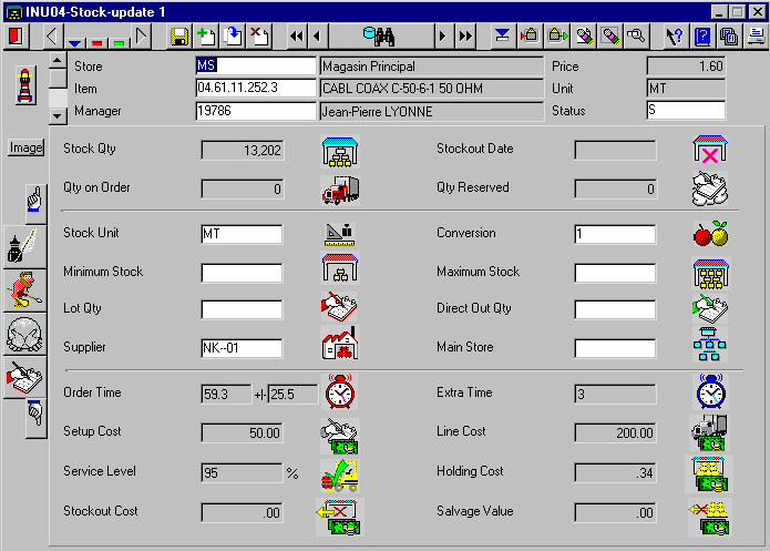
The purpose of this screen is to display, define or modify stock definition details.
FIELDS
| Store, Item | Store, Item. |
| Control | Item responsibility center/party or person, Manager |
| Unit | Unit of Measure UM, Basic Unit - this is the accounting unit. |
| Price | Sales price charged when the item is sold. |
| Status | Identifies events in the life cycle. |
| Stock Qty | Total quantity in stock, possible in different stocking locations or Binloc |
| Stock-out Date | For current stock-out, the date on which qty became 0 |
| On Order | Qty on order |
| On Reserved | Qty of currently not satisfied requests |
| Stock Unit | Default stocking unit |
| Conversion | Conversion factor between UM and stock unit |
| Minimum Level | Calculated or by constraint imposed logical minimum. |
| Maximum Stock | Maximum quantity that can be stocked or that one logical wants to hold in stock. |
| Lot Qty | Calculated or by constraint imposed logical set size or quantity. |
| Direct Out | User defined break quantity at which a material request normally will not be served from stock but turned into a special order. |
| Supplier | Default supplier from which the item normally will be reordered. |
| Main Store | Supplying store if current store is a satellite or transfer store |
| Order Time | Statistical order time of item by supplier |
DERIVED BY DEFINITIONS ACCORDING HIERARCHY:
Item (INU03)- Parameter Group (INU02) - Default value (INU01/1,2)
Service Level Service level in %
Holding Cost, Stock-out Cost, Salvage Value
Costs, calculated in the system currency
DERIVED BY DEFINITIONS ACCORDING HIERARCHY:
Item (INU03) - Parameter Group (INU02) - Default value (INU01/1,2)
Item, Group Transfer Channel (INU05/2) - Default value (INU01/3)
Extra Time Extra time component for orders and transfers
Setup Cost, Line Cost In system currency for orders and
transfers
NOTE: By pressing the <IMAGE> button, an image of the item is
displayed.
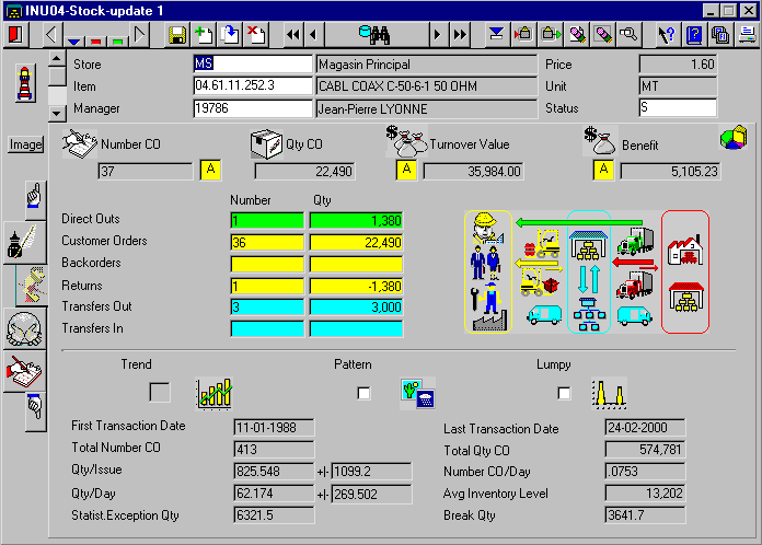
FIELDS
| CO | Number of customer orders |
| Qty CO | Total quantity CO turnover (issued - returned) |
| Turnover Value | Total amount CO |
| Benefit | Gross benefit = (Sales Price-Cost Price) x Qty CO |
| Direct Outs | Issues not from stock but as special orders directly from supplier |
| Backorders | Not immediately served demands |
| Returns | Returned |
| Transfers Out | Inter warehouse transfers out |
| Transfers In | Inter warehouse transfers in |
| Trend, Pattern, Lumpy | Sign and flags, see DEFINITIONS |
| First/last Transaction Date | Date first/last transaction |
| Total Number CO | All CO ever |
| Total Qty CO | All Qty CO issued ever. |
| Qty/Issue | Average quantity per demand |
| Number CO/Day | Average number of CO per day |
| Qty/Day | Average quantity demanded per day |
| Statistical Exception Qty | Statistical Exception Threshold |
| Break Qty | Break Qty or Exceptional Qty Threshold level |
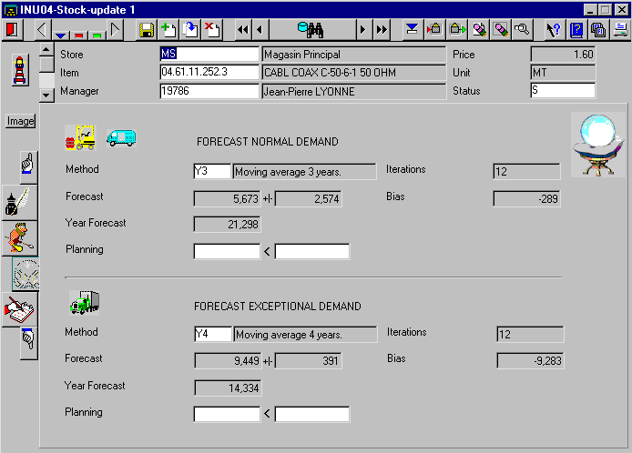
FORECAST NORMAL DEMAND
Expected total demanded quantity from stock, including issues, transfers
and returns. This quantity is important for stock re-order parameters.
FORECAST EXCEPTIONAL DEMAND
Expected total ordered quantity from direct orders, delivered directly
to the users, this quantity is important for contracts and non-stocked
items.
| Method | Forecasting method, which produced the best results - smallest average error or squared error - over the last (iterations) historical periods. |
| Forecast | Short forecast over by setup (MAU01) defined |
| +/- | Standard deviation or Forecast Error |
| Year Forecast | Forecast over year period - used for contracts and economical order quantity |
| Iteration | Number of historical periods over which the forecast method was tested (usually 12) defined in the setup (MAU01), sometimes less due to lack of history. |
| Bias | Average signed error, denoting systematical under or overestimation of forecast |
| Planning | User defined or by planning defined. IF DEFINED overrules the statistical year forecast. Value will be erased if <Date expires. |
< End of plan date, if DEFINED this date will when EXPIRED, ERASE the planning and its own value setting planning and date to undefined. Note: if UNDEFINED the planning definition will stay until by user action modified or erased.
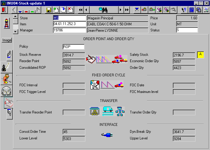
| Policy | Re-order policy: ROP - Reorder at reorder point FOC - Reorder at fixed order date MIN - Reorder at user-defined minimum to user-defined maximum |
| Stock Reserve | Average expected consumption in lead time |
| Safety Stock | Added extra term to overcome variations (larger than expected) consumption in the lead time |
| Reorder Point | Point (quantity) which triggers re-ordering: if available quantity in stock drops below this quantity, a reorder proposal is generated. |
| EOQ | Economic Order Quantity see DEFINITIONS |
| Consolidated ROP | ROP be temporary increased by consolidation conditions (see INU01 order constraints) |
| Order Qty | By logical constraints restricted EOQ |
| FOC interval | Review period between FOC dates |
| FOC Date | Next date at which an FOC order is triggered. Automatically maintained by the system. |
| FOC Trigger Level | FOC order line created on FOC date when quantity in stock below this level |
| FOC Max Level | Order line quantity calculated to fill up to this level |
| Transfer ROP | Transfer from main store, if quantity drops below this level |
| Transfer OQ | Transfer order quantity |
| Con Order Time | Time to calculated a target arrival date on the order receipt, the same for all lines on the order (same supplier, contract) |
| Dynamic Break | Break qty also taking actual stock situation in account |
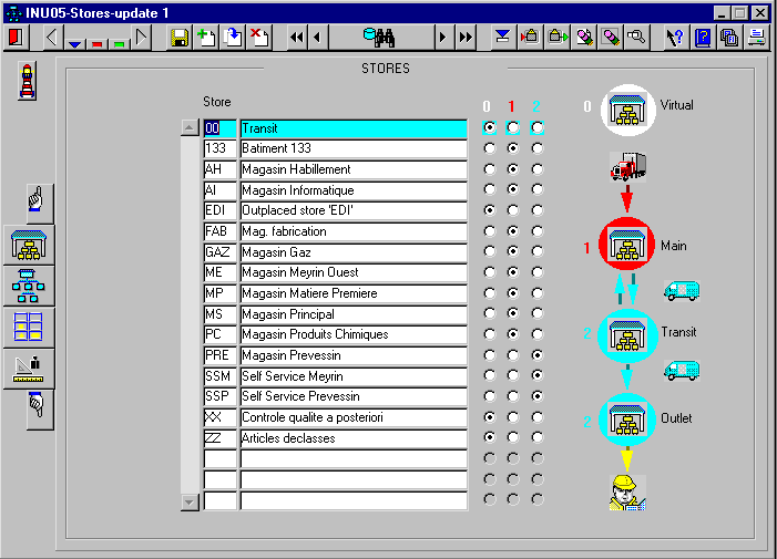
FUNCTION AIM
The purpose of this function is to define the different stores, store types, network definitions, transfer channels, stock locations, quantities and units.
FIELDS
Store Store code and name
Type Stores type:
0 = Virtual store is a logical or administrative store
1 = Main store is replenished by suppliers
2 = Transit or Outlet stores are re-filled by transfers from others
stores
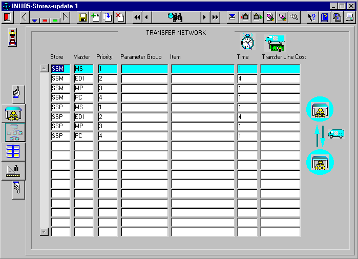
DESCRIPTION
This screen allows to define the transfer costs and times for transfers through the various transfer channels. The transfer cost and time can be specifically defined for a given item or parameter group, or can be more generally defined for a given transfer channel between a receiving store and a master - or providing store.
FIELDS
| Store | Satellite or detail store receiving the material. |
| Master | Master or main store supplying the material. |
| Priority | Order in which a transfer of items is attempted |
| Parameter Group | Group definition (see INU02), transfer channel is linked to the items of this parameter group |
| Item | Specific item for which transfer channel is defined |
| Time | Transfer time |
| Transfer Line Cost | Transfer line cost |
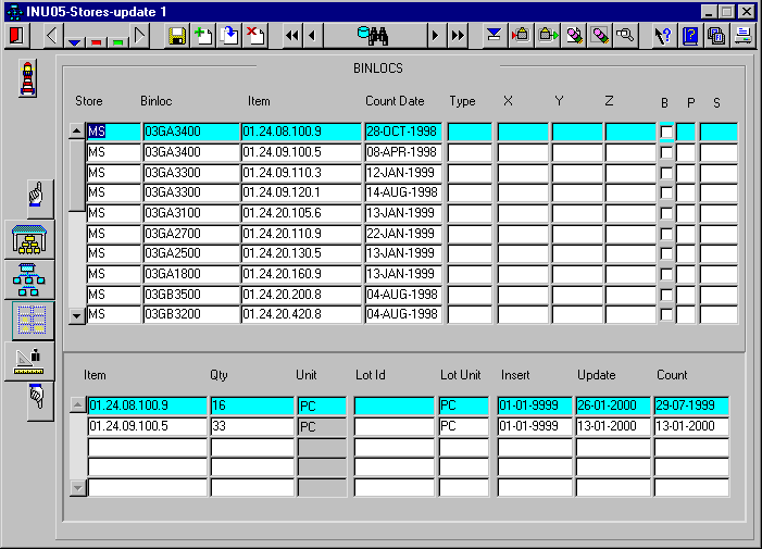
BINLOCS or STORES LOCATIONS
| Store | Store |
| Binloc | Store location code |
| Item | Item |
| Count Date | Date last cycle count (control of quantity) |
| Type | User-defined location type, like cooled, or heavy objects |
| X, Y, Z | Positional parameters, like path or alley, level or shelf, case |
| B | Blocked for picking, denotes that the location is temporarily blocked.
e.g. for counting purpose |
| P | Priority or pick first rule, e.g. caused by shelf-life |
| S | Sequence number, calculated to optimise picking route |
QUANTITIES
| Item, Qty, Unit | Item quantity in unit of measure |
| Lot Id, Lot Unit | Lot oritem identification (tracked items), stock unit |
| Insert | Put away date |
| Update | Last picking or change date |
| Count | Last cycle count date |
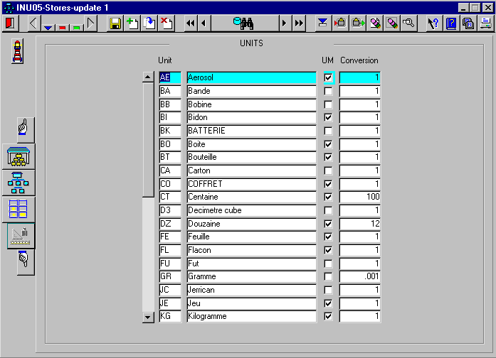
DESCRIPTION
This screen allows to define the units. Units can be used a basic unit or unit of measure, like kg, meter, litre, piece or more general like box, pallet, bottle
FIELDS
Unit Unique unit code and description
UM Checked if unit of measure
Conversion Relation to other units
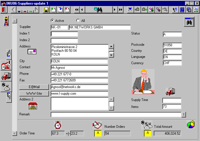
FUNCTION AIM
The purpose of this function is to define and modify suppliers.
FIELDS
| Supplier | Unique supplier code and short description |
| Index 1, Index 2 | User-definable indexes e.g. to denote type or classification of supplier |
| Status | Status |
| Address, City, Country | Address, City, Country |
| Contact | Contact person(s) |
| Phone, Fax | Phone number, Fax number |
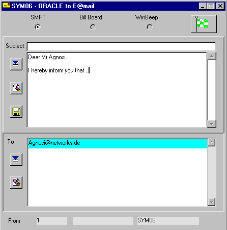
| E-Mail - pressing <E-mail> starts Email | |
| WWW-site | Web-site - pressing <WWW-site> starts the internet-browser |
| Supply time | Supply time |
| Comment | Short comment / remark |
| Items | Number of items currently supplied |
| Orders | Number received orders historical time window |
| Amount | Total amount received orders |
| Order time | Average order time |
| ABC | ABC Coefficients |
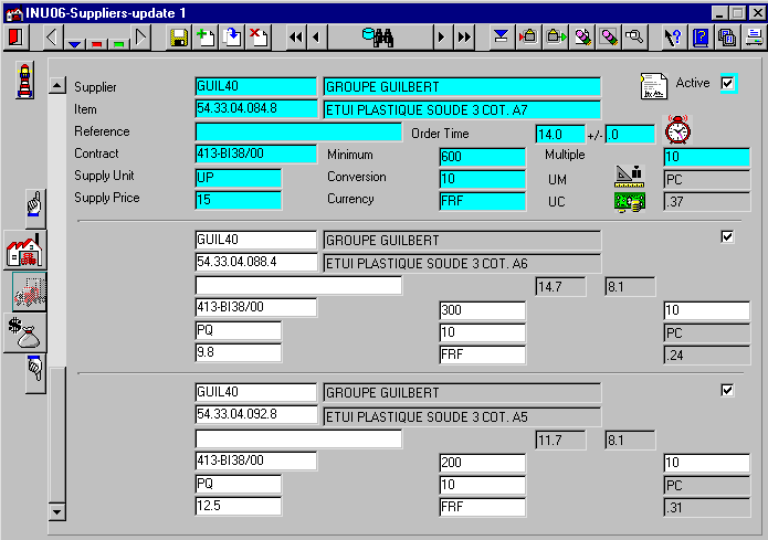
DESCRIPTION
This function allows to display, define and modify supplies, and historical supply conditions. Normally it is automatically maintained by interface, a historical record is created each time the active supply conditions change.
FIELDS
| Supplier | Supplier code and description |
| Item | Item code and description |
| Reference | Supplier code or name for item |
| Order Time | Historical order time |
| Contract | Contract |
| Minimum | Minimum order quantity in unit of measure (item unit) |
| Multiple | Multiple order quantity in unit of measure |
| Supply Unit | Unit supplier |
| Conversion | Conversion Supply Unit to unit of measure |
| UM | Unit of measure |
| Supply Price Supply Price | Supply Price in supplier Currency per Supply Unit |
| Currency | Supplier currency |
| UC | Cost price in system currency |
| Active | Denotes active contract |
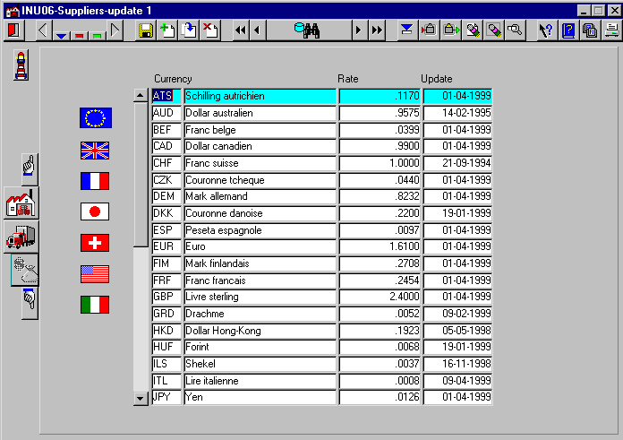
DESCRIPTION
This screen allows to define the currencies and rates.
FIELDS
Currency Currency type and description
Rate Exchange rate
Update Last modification date
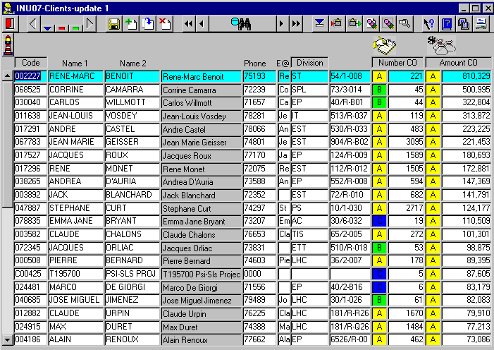
FUNCTION AIM
The purpose of this screen is to display, define, alter or delete customers.
FIELDS
| Code | Client code |
| First Name | First name |
| Last Name | Last name |
| Phone | Phone |
| E@ | |
| Company | Company, division or organisation |
| Office | Office location |
| ABC statistics | Number and total amount issued in history time window, and ABC classifications |
NOTE: if the <Code>, <Division>, <Amount> and <Number> header buttons are pressed, the order in which the data in the screen appears will change accordingly
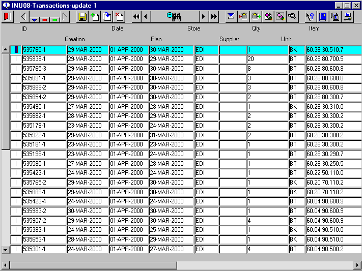
FUNCTION AIM
This function allows to display, define, alter or delete transactions.
HOW TO USE THE FUNCTION
Transactions should ONLY for simulation purposes in test-environment
be entered or changed. The transaction screen is wider then the window,
by using the <SCROLL-BAR> the screen will scroll and display the next
fields. In UPDATE mode, it allows to enter and modify transactions for
existing items. Entered positive quantity transactions will be treated
as issues with default type I. Negative quantities will be treated as
returns with default type R. In QUERY mode the screen can only be queried
and will display full information about the selected items and/or dates
and business events.
FIELDS
| T | Transaction type |
| ID | Transaction identification code e.g. Order Number, Issue transaction number |
| Creation | Date of creation, event creation date |
| Date | Event actual date. e.g. item issue date, purchase entry date, transfer date |
| Plan | Plan date. |
| Store | Store |
| Supplier | Supplier |
| Qty | Event Quantity |
| Unit | Unit of measure |
| Item | Item code |
| Index | Free user definable index e.g. Item class |
| Amount | Total amount in system currency at time of transaction |
| Client | Client code or identification |
| Company | Client organisation, company or division |
| Transfer | Transfer store, for inter warehouse transfers |
| Object | Object code, Equipment code for work orders, repair and maintenance |
| Location | Location of issue |
| Budget | Budget code |
| Stock Qty | Quantity in Store before transaction |
| Reason | Reason code for analysis purposes |
| Subtype | Many uses: Flag to denote back-order / Sub-Reason / etc |
The reason code is the only attribute that should be entered later, and allows to associate a reason to the event, for reporting and analyses.
EXAMPLES
Management information
Root cause analyses (maintenance, work repair cause analysis)
Observation - what happened
Direct Cause - cause
Indirect or root cause - 2e cause
Analytical accounting
Cost type/reason - type of - what happened
Cost budget - who pays
Cost originator - who cause
Reasons for Adjustments or Corrections of stock
Lost/missing when picking
Lost/missing when counting
Found when picking
Found when counting
Quality due to store (e.g. corrosion, dried out when
keeping too much too long)
Quality due to supplier (e.g. faulty technique)
Damage
Reasons for Returns
Wrong quantity due to requestor
Wrong quantity due to store
Wrong material due to requestor
Wrong material due to store
Quality
Damage
Delivered too late
TRANSACTION TYPES
The pop-up help screen or list of values shown below is available wherever an existing transaction type has to be entered e.g. for reporting or display of information or extraction of data to EXCEL.
It is an example of the many help-screens and lists of values available in the system
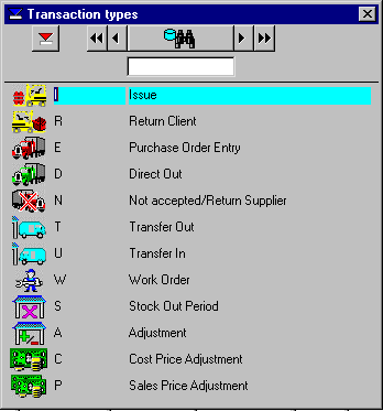
The following transaction types are supported
I = Issue of material by client order
D = Direct Out of client order by special purchase order
R = Return of material by client order
A = Adjustment or correction stock quantity
P = Sales Price Adjustment
C = Cost Price Adjustment
E = Entry of ordered material
T = Out going inter warehouse transfer
U = Incoming inter warehouse transfer
N = Not accepted order reception, return to Supplier
S = Stock-Out time
W = Work Order
INU09 - Control Centers, Managers
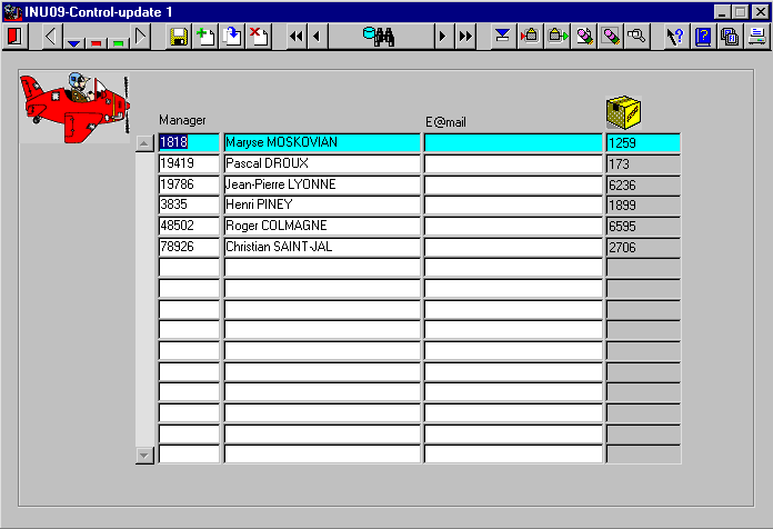
FUNCTION AIM
The purpose of this screen is to display, define, alter or delete item control or responsibility centers.
FIELD
Code Responsible party, person or manager code
Description Name or description
E-mail E-mail address
Item Number of items
FUNCTION AIM
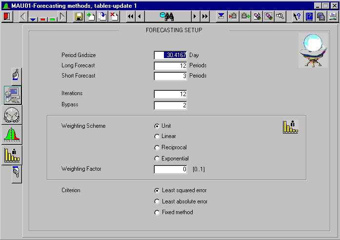
The purpose of this screen is to define the initial forecasting set-up. These parameters should normally not be changed anymore.
FIELDS
| Period Grid size | The length of the time interval for which the historical demand is sampled and the forecast is calculated. |
| Long Forecast | Number ofperiods long forecast to calculate re-order quantities and contract conditions |
| Short Forecast | Number ofperiods short forecast to calculate re-order triggering conditions |
| Maximum Number Iterations | The number of periods in the past for which the real historical consumption and the forecasts are compared. The forecasting methods are evaluated by testing the fit to the real historical quantities |
| Minimum Number Iterations | Minimum number of tests for a forecast formula, if there is not enough history for a formula to perform the specified minimum, the formula is bypassed. |
| Weighting Scheme | A weighting scheme may be applied to the tests, aimed at increase of the accuracy, giving more significance to the most recent tests or deviations between forecasts and historical periods |
| Weighting Factor | Factor applied in the weighting scheme |
| Best Fit Selection Criterion | Optimal method selection as best fit to: 1 = Least average squared error <E2> 2 = Least average absolute error <|E|> 0 = No selection, fixed method |
HOW TO USE THE FUNCTION
This function displays information about the forecasting set-up. By pressing <TAB> buttons one can reach the next pages.
DESCRIPTION
Whatever would have worked best in the recent past should be used to
predict the future.
A large number of different forecasting strategies is used simultaneously
to forecast a number of recent historical periods of demand. Each formula
is measured according to the variance from what actually happened in the
know past, and the formula which worked most accurately, is selected and
used to predict the future.
BENEFITS
The forecasting uses a multi-method procedure simultaneously calculating a large number of forecasts for a number of historical periods, using a large set of different forecast methods or formula (defined in MAU01/2), and subsequently selecting the method best fitting to the historical consumption for each individual item. By dynamically choosing the method giving the best fit to the historical consumption one ensures that:
The forecast F will automatically adjust to sudden changes of the consumption pattern (sudden rise/fall of demand) by selecting the best fitting method to accommodate these changes.
The method with the best fit, gives also a good estimate of the deviation or error of the forecast. This deviation D is an important factor in many calculations: it gives not only an estimate of the accuracy of the forecast, but it also gives the different probabilities that the reel consumption will take the values F+D or F+2D, etc. (Forecasting actively uses D)
The average error <E> or bias gives a good indication of the
offset or tendency of the historical demand to grow/diminish.
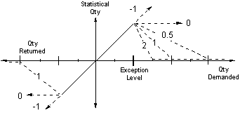
The statistical used consumption includes customer returns, and a weighted fraction of the exceptional demanded quantities. Set-up allows to complete/partial/not including a fraction of the exceptional demand by the Exception Filter.
The exceptional demand is defined as demand for quantity larger then the break quantity calculated by parameters defined in INU01 or user defined as constraint direct-out level INU04
Although the number of exceptional large demands is only a fraction of the total number of demands, the total exceptional quantity may outweigh the total normal demanded quantity. Sometimes it is possible to satisfy an exceptional large quantity from stock without endangering the serving of the normal demands. Sometimes a fraction of the exceptional large demanded quantity is served from stock and the balance is served by direct out. Including a fraction of the exceptional demand will normally reduce the forecast error. Exception Filter setting:
-1 Take the total exceptional quantity for statistics
0 Take as fraction the exceptional threshold level
1 Decrease the fraction taken for statistics if the quantity
For every forecast method a number of coefficients Ci can be defined in RPU05, such that a forecast for the next period can be calculated, expressed in the coefficients and the periods.
Forecast F by method m for the next period P
Fm (P) = Sum (Cm(i) x Pi )
The setup provides a number of standard methods and coefficients.
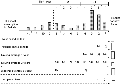
The period trend in the example, is calculated as the last period, plus the difference from the previous period: P1 + (P1 - P2) = 2 x P1 + -1 x P2
NOTE: Due to negative coefficients and/or user returns the forecast may become negative.
if the switch Allow negative Forecasts = Y. Allowing negative values of the forecast will make the test for the best fitting method more critical (One 0 is much alike to another 0, if no negative values are allowed).
CHOOSING THE BEST METHOD
The different forecast methods can be tested, how well they would have produced a forecast of the last N historical periods P1 ... Pn or Maximum Number Iterations N, by calculating the historical consumption R(P1 )... R(Pn) and forecasts for each forecast method m Fm(P1 ) ... Fm(Pn) over the last N periods and calculating the difference or fit of each method to the historical consumption.
The number of iterations must be chosen sufficiently large to reduce forecast error. It does so because it reduces formula selection on random change. A formula may be accurate once by accident, but may not stand the test of a large number of iterations. A too large number of iterations may decrease the accuracy, because it focuses the test on the fit to history of the far past.
The recommended default for the setup parameter Maximum Number Iterations is 12.
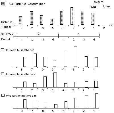
If there is not enough history for a formula to perform the specified number of iterations, it may run with a lower number of iterations. If the number of iterations is less then 3 it is bypassed altogether.
To test each method, the differences E between the real R consumption and the forecast F for each method m are calculated: Em(P1) = Fm(P1)-R(P1) ... Em(Pn) = Fm(Pn)-R(Pn)
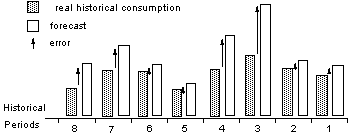
For each method the average error, average absolute error and average squared error are defined as
<Em> = 1/(N-1) x Sum ( Em(P1) ... Em(Pn) )
<|Em|> = 1/(N-1) x Sum ( |Em(P1)| ... |Em(Pn)| )
<Em2> = 1/(N-1) x Sum ( Em(P1) 2 ... Em(Pn) 2 )
Where N is the number of actual iterations.
For random errors <Em> is near to zero. A large value of <Em> is caused by a systematic offset or trend between the predicted and real values. The value of <Em> is taken as TREND factor Tm for the method m, one advantage of adding Tm to the forecasts Fm is that all errors are reduced and the fit is improved.
the predictions Fm(P1)+Tm ... Fm(Pn)+Tm are compared with R(P1) ... R(Pn), and <|Em|>, <Em2> are calculated ( <Em>= 0 is per definition )

The best to fitting method or the method with the least error can now be selected as the method with the smallest value of <Em2> or <|Em|>. For this method we can obtain for the next period an estimate Fm(P0) with error <|Em|> and trend Tm.
Set-up allows both the fit to <E2> or <|E|> as best method selection criterion.
(<E2> is general accepted as best criterion, sometimes <|E|> is preferred for noisy data...)
The set-up also allows a weighting scheme to be used, to focus the method fit on the most recent periods:
<E2> = N/(N-1) x Sum W(i)*E2(i) / Sum W(i) where E2(1), is the squared error of the most recent period, E2(2) the next, etc., (same for weighted <|E|>)
FORECAST SCHEDULE
If a schedule of one forecast period is used, for the recommended Periods/Year
= 4 setting
an accurate estimate for the NEXT 3 MONTHS is obtained for:
DEVIATION
TREND
DEVIATION is used in the calculation of the stock safety SS
an estimate of the forecasted year consumption for normal demand from stock for non-seasonal items is given by
YEAR ESTIMATE = 4 x FORECAST + TREND x W(I) + Deviation Factor x 2 x DEVIATION
with a lower limit of Deviation Factor x 2 x DEVIATION
The lower limit is imposed because the forecast can never be more accurate then the deviation or error itself. The total error of the year estimate as square root (4 independent errors) = 2 error of one forecasted period. The factor W(I) depends on the number of real iterations (between Minimum Number Iterations and Maximum Number Iterations).
For seasonal items a full year schedule of the next 4 periods is calculated and 4 x FORECAST in the formula is replaced by FORECAST (P1)+(P2)+(P3)+(P4)
Note: Full year forecast schedules can be obtained if the setting Forecast
Schedule Periods is set to Periods/Year.

DESCRIPTION
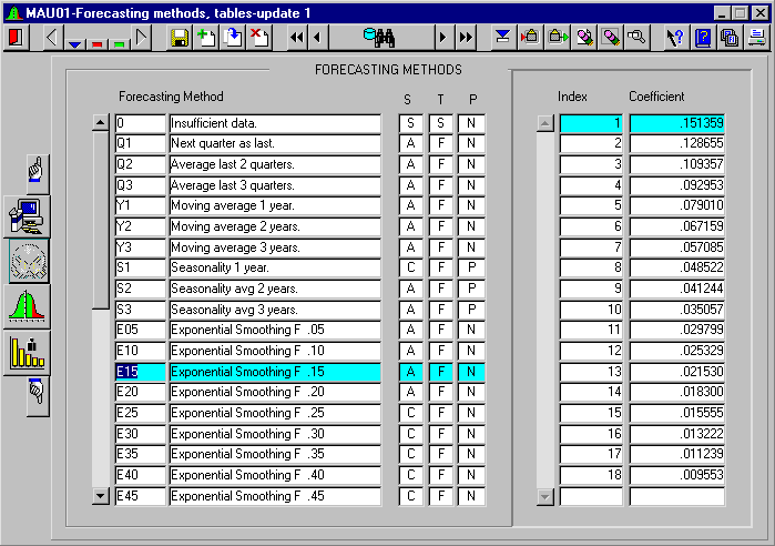
Forecasting allows any number of methods, to be defined. The purpose of this screen is to define, de-activate, alter or delete Forecast Methods.
FIELDS
| Id | Unique code of forecasting method. |
| Description | Short description of forecasting method. |
| S | Status: A = Active, C = Not Active. |
| T | Type: F = Forecasting method, L = Life cycle pattern |
| P | Flag: P = Seasonal pattern, N = No seasonal pattern |
| Index | Coefficient number. |
| Coefficient | Coefficient Factor. |
HOW TO USE THE FUNCTION
New forecast methods can be entered by pressing <CREATE RECORD>.
In the next block the coefficients for the entered method can be defined or modified. A forecast method may be removed by pressing <DELETE RECORD> when the method is in use a warning is issued. When <COMMIT> is pressed after this warning, the method definition will also be erased from the items using the deleted method.
MAU01 /3 - Mathematical Tables
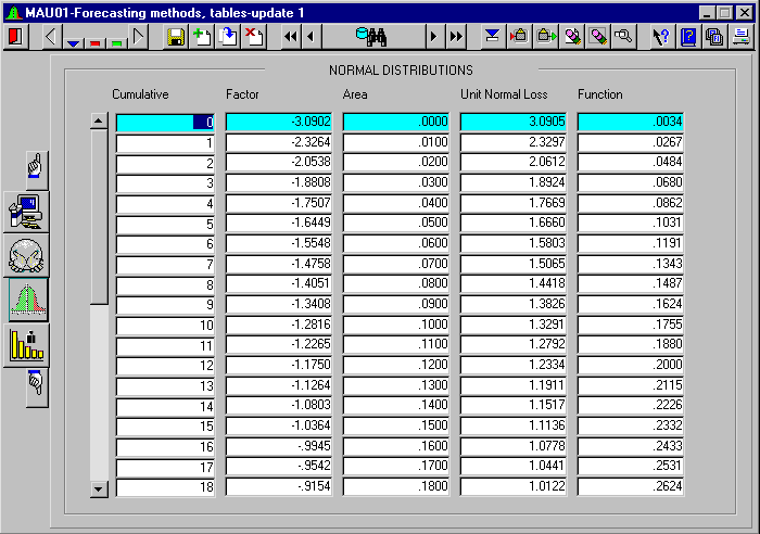
THE MATHEMATICAL TABLES
FIELDS
| Cumulative | Cumulative Probability P(Z) in % Level as approximation of the area under a Standardised Normal Distribution. This table will be used in calculations if the Real Distribution is not available (see Operations Manual) |
| Factor | Z Factor -Factor relating the service level and Standardised Normal distribution and Unit Normal Loss Integral |
| Area | Cumulative Probability P(Z) |
| Unit Normal Loss | E(Z) Factor relating the Unit Normal Loss Integral |
| Function | F(Z) |
BALLOU page 667 Standardised Normal/page 668 Unit Normal Loss Integral
Silver and Peterson page 699 Gu(k) represents the Unit Normal Loss Integral
(see also P 271)
HANDBOOK of MATHEMATICAL FUNCTIONS M. Abramowitz and I. A. Stegun
page 966-972, Page 976 table 26.5 , Page 3 pi = 3.1415 92653 58979
FACTOR = Z
P(Z) = (1/sqrt(2*pi))*exp(-1/2*power(Z,2))
AREA = integral -00 to Z over P(Z)
NORM_FUNCTION = exp(-0.5*power(NORM_FACTOR,2))/sqrt(2*3.141592654)
DESCRIPTION
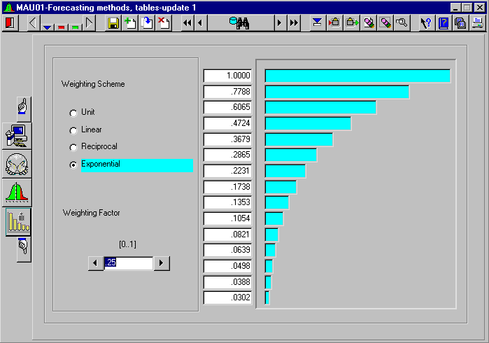
This screen displays graphical and numerical results of the various weighting schemes, one may choose a weighting scheme and calculate weights changing the weighting factor over its range of allowed values.
WEIGHTING SCHEMES
Weighting Scheme W, Weighting Factor F
Unit: W = 1, No weighting
Linear: W = greatest ((Factor-Y), 0)
Reciprocal: W = 1/(1+greatest ((Factor xY), 0))
Reciprocal: W = exp (- Factor xY)
AIS
Webmaster