May 14, 19978Advanced probability theory as basis for accurate estimates

of safety stock

(Demand rate versus a single demand approach in inventory control)

Patent pending

B. SCHORR and M. KREVER

Summary

The concepts of probability theory have been applied to derive an accurate expression for the buffer stock quantity necessary to meet a pre-defined service level. The proposed method is not based on exponentially smoothed MAD, rules of thumb and classification of items in categories (ABC, Segmentation, etc..), or an estimate by summing a single-period demand distribution over the length of the lead time, but a complete mathematical solution based on the real statistical distributions. A general and complete theory is derived below which covers the general concept wherever stock is placed as a buffer between supply and consumption. The theory developed is both applicable to Q-System as well as P-Systems and leads to exact expressions for the reorder point and safety stocks in relation to customer service. Practical results show that the proposed method enables a significant enhancement in the service level, while reducing the average value of the stock.

1 - Introduction

Today's market increasingly demands the development and availability of products with high quality, short delivery times and costs which mirror real market situations. The very large economical penalties of downtime and off-spec production require all necessary resources to be available at the required time, in the quantities demanded and at the lowest cost. To this aim optimal management of the resources availability is necessary.

The resources availability is controlled by parameters which have to be determined using customer service requirements and historical stock data. In books on practical applications and in commercial systems the key data used to determine these parameters is the expected demand rate D (quantity per unit time interval) and the variance thereof. For a low demand rate, the accuracy of the calculated demand rate depends heavily on the choice of the unit time interval. Particularly sensitive to the choice of the unit time interval is the estimation of the variance of D.

In this paper another approach is proposed which is based on single demands Q during lead time L (time between ordering and arrival of material). This method is more natural and has many advantages compared to the demand rate approach. In section 3 fundamental formulae are derived. In section 4 approximations are derived for both approaches in parallel for easier comparison. In section 5, simulations based on real data of the CERN stores will underline the advantage of the single demand approach. Section 2 recalls the main concepts, definitions and equations for the customer service S and reorder point R.

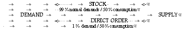
Customer demand is often not known in advance, and can exhibit large fluctuations over time. Long and varying lead times often preclude providing the demanded items by direct ordering of the supplier. Direct availability of demanded items can only be ensured by keeping an item stock as buffer between supply and demand.

DEMAND <- STOCK as BUFFER <- SUPPLY

To assure serving demand for items from stock, items must be re-ordered to replace materials which have been issued, or which are known to have future requirements.

In practice two basic stock keeping policies can be distinguished:

Q-system: Re-order an economical quantity at a certain stock level the re-order point R, which ensures serving of demand during the lead time L. This method has the major benefit of the just in time, most economical re-ordering, of each item individually.

P-system: Re-order at periodic intervals in time P an order quantity such as to refill the item stock to a pre-defined maximum stock level M, which ensures availability over the time interval P+L. This so-called fixed order cycle or periodic review policy has the advantage that an ensemble of items for the same supplier can be ordered together, and that the moment of the order is known in advance.

For both Q-system and P-system policies it is reasonable to formulate a certain quantity, the exceptional quantity threshold or break quantity, above which a demand is not served from stock, but turned into a special order, the so-called direct-out.

In this way unusually large single demands, which would otherwise lead to stock-outs and dominate the statistics, can be filtered out.

Example: Only few demands (less then 1 %) may contribute to more then 50 % of the consumption.

Although the outliers are removed by using the break quantity criterion, the lead time uncertainty and the variability in number and size of the normal demands has as consequence that the consumption is variable, and can only be predicted with a certain probability, and thus the parameters R and M can only be determined in a statistical sense. The values of these parameters however, are very critical for successful stores management.

Good inventory management involves balancing the product availability, or customer service, on the one hand with costs of providing a given level of product availability on the other. Too high estimates of the parameters will result in high stock values and overstock, while too low estimates will result in frequent stock-outs and low customer service. If some parameters are set too low and others are too high, a high stock value in combination with a low customer service will result.

The re-order point R for Q-systems and the maximum stock level M for P-systems are calculated in exactly the same way, the only difference being that R depends on the lead time L whereas M depends on P+L, with P being the time between two periodic reviews. Therefore, the equations are explicitly discussed for the re-order point R only.

The value of the parameter R is expressed as the expected consumption E(X) over the lead time L , to which an increment of inventory, the so-called safety stock is added to overcome the larger then expected demand and reduce the risk of stock-out. This incremental inventory component is a function of the variability Var(X) of the consumption X , and the desired customer service S.

It is assumed that the demand X during lead time has a normal distribution with mean E(X) and variance Var(X). Then, the re-order point is set equal to

where z = G^-1(1-p) (G being the distribution function of the standardized normal distribution) is chosen in such a way that only with probability p there is more than the reorder point R demanded quantity during lead time thus ensuring a customer service of at least S = (1-p)x100 % of the cases.

Assuming the errors to be normal distributed the variance Var(DT) for another period T can be readily obtained by the equation Var(X) = (L/T) Var(DT).

If both the lead time L and the demand rate D are independent random variables the following definitions are commonly used [5]

Two basic methods to derive Var(DT) can be distinguished

1. Demand variance based on mean average absolute forecast deviation MAD

This method is the most frequently used forecasting method and is based on a measure of the difference between old forecasted consumption and the observed consumption.

Absolute error = | actual demand - old forecast |

Weighted average, or exponential smoothed average is taken to calculate new MAD values.

new MAD = alpha x Absolute Error + (1-alpha) x old MAD

Traditional a factor 1.25 is added to correct for the fact that one theoretically wants to use an estimate of the standard deviation or standard error

standard deviation = Sd = 1.25 x MAD

The MAD is actually rather an estimate of the goodness of the fit of the forecast method used, then an expression of the variability in demand. Different forecasting methods will in general result in different forecasts, and thus in different MAD values.

2. Demand variance based on the single period demand distribution (SPD)

This method is based on a direct measure of the real variance of the historical data. The historical demand is sampled in a number of intervals i from which a single period demand SPD distribution can be constructed by ordering by size and frequency of occurrence, and of which the standard deviation can be obtained directly.

Both methods 1 and 2 strongly depend on the sampling of the total demand in intervals

That the sampling of the demands in intervals or periods of consumption leads to actual loss of information contained in the historical data, will be illustrated below, by use of a number of simple representations.

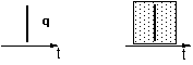
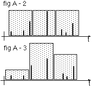
A demand for a quantity q will be represented by a bar |, the quantity for a certain period is presented by a box

Below two demand patterns are represented Fig A-1 and Fig B-1:

the look very different, in the classical presentation, sampling the quantities in periods however, may completely fail to recognise the difference as depicted in Fig A-2 and Fig B-2

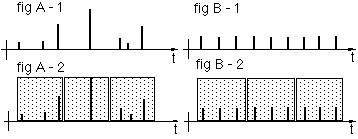
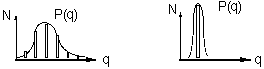
While the details of the individual demands are masked in the qty/period distribution in fig A-2 and Fig B-2, it can be seen that quantity per single demand distribution of the two demand patterns are clearly different: one is broad, the other is sharp

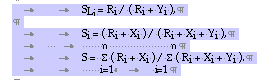
Moreover a qty/period distribution is prone to errors: a small shift of the sample periods to the right or to the left may lead to a completely different distribution, for the same demand pattern in time: see Fig A-3, which can be derived from Fig A-2 by a small shift in the sampling grid. (Note: a higher density of grid points may not resolve this problem: it will generally lead to a large number of accurate, but meaningless zero quantity samples)

A third method, based on mathematical probabilities using statistical distribution functions, not hindered by the observed inaccuracies of the 2 methods described above, will be derived below.

However, first definitions of service levels for customer service must be given, which are key factors in the determination of the success of the different methods.

2 - Customer service, service level S and the re-order point R

The natural way to define the service level for one item or a group of items in a store during a time interval T is given by the expression

another related commonly used criterion depends on the served number of demands rather then the served quantity

Where (2.1) is related to the quantity and hence is directly related to the profit of consumer goods, the criterion (2.2) is rather related to serving or not serving events and the costs of stock-out, like in demands for spare parts.

It should also be noted that the concept of the a priori service level has a number of different interpretations. Whenever managers speak about the desired service level, they normally mean, the overall or global service level, while logisticians usually interpret it as service level in the lead time. Analysts will, aposteriori, obtain the global values of (2.1) and (2.2) from historical data, regardless of lead times.

The service level depends on the re-order point R (and the ordered quantity which will not be considered here in detail) and can therefore be influenced by the choice of R. The larger R is, the higher is the service level, of course the higher is also the cost of the store. It is therefore important to choose the re-order point rather carefully.

Suppose the time interval T on which S depends is in the future, then S is a (discrete) random variable, whereas if T is in the past the value of S is determined;

in probabilistic terms, in the latter case, its value is a realization of the random variable S.

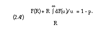
Before continuing to discuss the service level and the re-order point, it will quickly be shown why for the determination of the service level over a longer interval it is sufficient to determine R such that the service level during lead time has a certain value in order to guarantee at least this value for the whole interval T.

Let the time interval T be the sum of n cycles where each cycle has the length between the arrival times Ti-1 and Ti of two consecutive orders of an item. Let Si be the service level during the i-th intervals [Ti-1, Ti). In addition, let SLi be the service level during lead time Li in the i-th interval [Ti-1, Ti). Let finally Ri be the re-order point during the i-th interval, Ri + Xi be the demanded quantity during the i-th interval which was satisfied and Yi the unsatisfied demand during the i-th interval. With these notations the following holds:

With these formulae it is easy to show that

Therefore, if SLi has a certain value, Si and S have at least the value of SLi. In general, they will be better. It therefore is sufficient to concentrate on the choice of SLi.

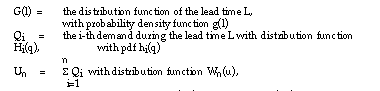
Suppose that lead time L and the demanded quantity during lead time are known. In this case R can be set equal to the demand during lead time to warrant a service level of 100%. However, normally lead time and the demand during lead time are unknown, and therefore the choice of R has to be made under uncertainty. There are several ways to define an equation to determine R. Three of them are mentioned here.

The derivation of the first equation is based on the concept of a confidence interval. Let p be a small probability (e. g. 0.05), R will then be chosen such that a given service level sp (say 90% or more) will be guaranteed during lead time with probability 1 - p. The equation to determine R reads

The second equation is the limiting case of equation (2.2) for sp = 1.

The third equation consists in determining R such that the expectation of S has a certain predetermined value s, for instance s = 1 - p:

In order to have more explicit equations for R, the following notations are introduced:

Since by definition of R the quantity Qser = min(R, Qtot), the service level S during lead time L can be written as

Therefore,

from which follows for the equation (2.2):

Finally, using (2.4) and (2.5) in equation (2.3), the following equation is easily obtained:

It is clear that each of the equations (2.3') and (2.4') leads to another solution for R. The most convenient equation is (2.3') for sp = 1. It leads to the largest value of R and yields therefore the most conservative solution. It is always used in the applications. Both equations depend on the distribution function F of Qtot. Therefore, in this connection, it is necessary to obtain at least an estimate of F. This is discussed in section 4.

3 - Explicit formulae for the distribution function F(s;R)

Before approximate formulae for F(s;R) are considered, explicit expressions are derived under different assumptions. For this purpose, the service level as defined in (2.1) is written as a ratio of sums of single demands during lead time:

where UK(L) = the quantity served during lead time L and UN(L) = the total quantity demanded during lead time L.

The following notations are introduced:

In order to determine the distribution function F(s;R) of S in equation (1.4), the quantity Pr(S s) is calculated. The use of conditional probabilities leads to the expression:

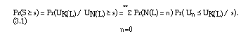
To work out the right-hand side of equation (3.1), the probability Pr(Un _ UK(L) / s) is evaluated first. The following equivalent events are used:

The random variable UK(L) takes two different values, depending on the values of Un.

The following holds:

Owing to s 1, equation (3.2) can therefore be written as

Therefore, equation (3.1) becomes:

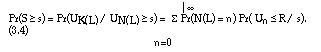
This yields an expression for F(s;R) = 1 - Pr(S s) without any further assumption, but at the same time showing the dependence of F(s;R) on R and s in an explicit way.

In order to arrive to more explicit formulae which still match real systems reasonably well, the following assumption is made:

Assumption (i):

Let

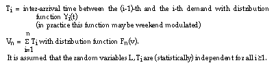
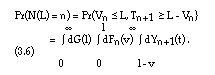
Under this assumption, Pr(N(L) = n) on the right-hand side of equation (3.4) can be evaluated more explicitly. For this purpose, the following equivalent events are considered:

for L=l. The equivalence of both events in equation (3.5) is easy to see when considering the definitions of L, Vn and Tn+1, given above.

Using the notations introduced above, the following equation is obtained:

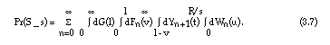
Insertion of equation (3.6) into equation (3.4) and using the distribution function Wn(u) of Un leads to:

In order to arrive at even more explicit expressions, another assumption is added.

Assumption (ii):

The Ti have the same exponential distribution with probability density function (pdf):

It can easily be shown that, under assumption (ii), the random variable Vn follows an Erlang distribution with the pdf

Using (3.6), (3.8) and (3.9) leads to:

which shows that N(l) follows a Poisson distribution.

Using (3.6) and (3.10), equation (3.7) can be written as

keeping in mind that this formula is only true under the assumptions (i) and (ii).

It should be mentioned that if the Qi are statistically independent and have a probability density w(u), then dWn(u) = wn(u) du in equation (3.15) and wn(u) is the convolution of the densities of the Qi and, if the Qi have the same pdf w(u), wn(u) is the n th autoconvolution of w(u).

The probability density function of U , p(u) is given by

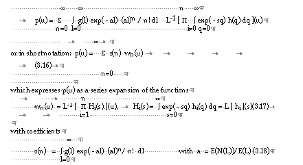
Although no general explicit expression exists for the convolutions wn(u), the equation (3.17) can be solved analytically, for a limited number of probability distribution functions, like the normal and the gamma distribution, allowing exact solutions for the series (3.16) to be obtained.

If the demand density is very low, the first coefficient (3.18) will dominate the series expansion, and p(u) will resemble hi(q). In the expression (3.16) for p(u), the r(n) can be replaced for other time rate functions, for instance when the inter arrival time is dependent, or a function of time, like failure rates described in the mathematical theory of reliability [1].

For larger demand densities where the series is dominated by the first 3 terms, p(u) will become skewed. For a large demand density, the approximation of (3.16) by a normal distribution is reasonably accurate, owing to the central limit theorem of statistics. For a low number of demands during lead time, p(u) can be expected to be nearly normally distributed, only if the distributions of hi(q) are nearly normal.

An important feature of the use of the break quantity condition, is that it tends to take existing skewness away from hi(q), transforming the hi(q) to a more normal distribution.

Although there exists no explicit expression for the convolutions wn(u), the expectation value E(U) and variance Var(U) of p(u), equation (3.16) can be readily obtained, as shown in the next paragraph.

4 - Approximation formulae for the distribution function F(s;R)

The quantity Qtot may be represented as a sum of certain sub-demands. Two different ways will be considered, for comparison of the single demand with the demand rate approach.

For this reason, the following concepts and notations are used:

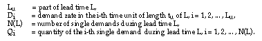
Then, the following two representations of Qtot are considered:

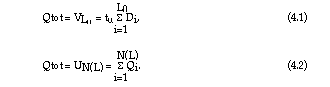
It should be noted that for historical reasons Di is defined as a rate. In the literature on practical applications the sum (4.1) is normally written as Qtot = L D where D is the demand rate per time unit with the drawback that the formula for the variance used for Qtot does not correspond to this product but to the one which will be derived later for the sum in (4.1).

With respect to the random variables L, Di, N(L) and Qi. the following assumptions are reasonable:

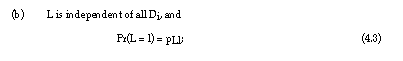
The time intervals between two single demands are independent and have the same exponential distribution q with

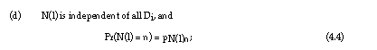
where a is the number of single demands per time unit. In this case it can be shown (see for instance [1]) that N(l) has a Poisson distribution with

In practical applications (see for instance [2], [5]), the distribution function F of Qtot is approximated by a normal distribution with mean m = E(Qtot) and variance s² = Var(Qtot).

Owing to the central limit theorem of statistics, this approximation is reasonably accurate if E(L) and E(N(L)) are large. For a low number of single demands during lead time, Qtot can be expected nearly normally distributed only if the distributions of D and Q are nearly normal, and can be used to calculate an approximate Rapp.

This equation for single demand distributions is the counterpart of (1.1).

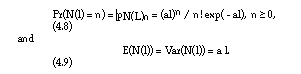
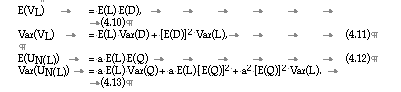
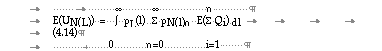
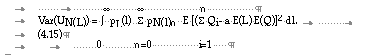
In the following the expectations and the variances of VL and N(L) are evaluated under the hypotheses (a) to (e) above and the assumption that N(L) follows a Poisson distribution with mean and variance as given in equation (4.9). The results are summarised first for comparison, the derivation of the results follows.

The derivation of these formulae is as follows:

from which equation (4.10) follows.

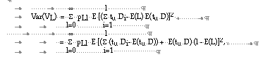
from which equation (4.11) follows using assumptions (a) and (b) above.

Using assumptions (c) to (e) and equation (4.9) in (4.14), equation (4.12) follows.

Using in (4.15) the equation (4.9) and

finally leads to (4.13).

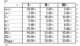
For illustration of the accuracy of the approximate expression Rapp, two examples of the exact determination of R are considered below, for the single demand approach, for two different probability distributions where exact solution is possible. Comparing R1 and R2 with Rapp shows the approximation Rapp to be close to the true values in both cases.

Example (1) the normal probability distribution

Suppose that the assumptions (a) to (c) are satisfied, that L = l is known, N(l) follows a Poisson distribution, and that the Qi have the same normal distribution with mean m0 and standard deviation s0. In this case, in equation (4.6), the integral over l disappears since L = l is known, pN(l)n is given by equation (4.8), and pQn is the density of a normal distribution with mean nm0 and standard deviation s0. Let sp = 1, with equation (4.6) and the facts which were just mentioned, equation (3.2') then becomes:

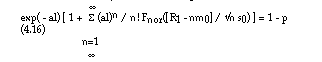
where Fnor is the distribution function of the standardised normal distribution.

Before numerical values for m0, s0, l, a and p are considered, a second example is formulated.

Example (2) the gamma probability distribution

In this example the assumptions are the same as in example 1 with the only exception that the Qi have a gamma distribution with the probability density function

with m0 = b'/a' and s0 = _b'/a'. In this case pQn has a gamma distribution with E(Un) = n b'/a' and Var(Un) = n b'/a'². In this case, equation (2.2') for sp = 1 becomes:

Finally, since in both examples E[N(l)] = a l, the method which approximates the distribution of UN(l) by a normal distribution with mean and variance given by the equations (4.12) and (4.13), respectively, yields:

The following results have been obtained for p = 0.05 and different parameter combinations:

Test of the different methods

In order to judge the performance of different sets of reorder points, calculated by the different methods, to produce desired service level, a number of criteria to measure their success can be formulated.

For individual items the following definitions (2.2) and (2.1) have been given

SL1 (item) = number of demands served/total number of demands

SL2 (item) = value served/total value = quantity served/total quantity

For a set of items the following overall criteria can be defined

SL1 = demands served (all items) / total number demands (all items)

SL2 = value served (all items) / total value (all items)

SL3 = average SL1 (item) +/- deviation SL1 (item)

SL4 = average SL2 (item) +/- deviation SL2 (item)

|E3| = average error | SL1 (item) - desired SL(a-priori)|

|E4| = average error | SL2 (item) - desired SL(a-priori)|

ROP value = sum over items ( R x price )

Average stock value = sum over stock changes ( time x stock x price ) / sum (time)

In real life the success of the logistics parameters is often interpreted as a high observed service level in conjunction with a low average stock value. There are however many factors which may influence these results. Order quantity consumption, changing order policies, changing lead times, changing demand patterns, handling policies like splitting of back orders, order of serving, definition of break quantities, are a number of factors.

Larger order quantities will result in larger consumption times and lead to very few reorder events, if lead times change as result of change in order policies, or change of supplier, shorter and less variable lead times may result in a lower stock and higher service levels, even if the parameters are calculated less accurately.

Therefore a specific test simulation has been devised, aimed at testing the success in fulfilling the service level conditions, excluding all other influences as much as possible.

At the start of the simulation the quantity on stock is set equal to the reorder point, historical demands are served from the stock, or not served if the stock is empty. Unsatisfied requests are not backordered. After a lead time has passed the quantity on stock is restored to R, while the process of serving demands continues. Ever after the stock is re-set to the reorder point after a lead time has passed. In this way, the whole simulation run will consists of lead times only. The full serving history is kept and can be analysed after each simulation. The results still depend on the order of serving, splitting of the backorder, and break quantity used.

Order of serving: For the same items, the order of serving is such that the requests for small quantities are served first. If there are many requests for the same item, this ordering will lead to the situation that the request for the largest quantity, which has the highest possibility of creating a stock-out, will be served last.

Splitting of backorders: If the quantity on stock is insufficient to serve the quantity requested, the total stock may be served to satisfy at least a part of the quantity requested, while the balance is served later on arrival of ordered material. The resulting stock-out will lead to unsatisfied requests for much smaller quantities, which could have been served otherwise. Non splitting will in general lead to higher serve levels, where smaller quantities are served more often.

In the simulations described below, ordered serving in combination with splitting of backorders is used.

Normally an extra quantity is added to the reorder point R to compensate for the fact that the statistical consumption does not start at the exact value of R, but when the reordering is triggered by a demand, the quantity on stock can drop significantly below the reorder point.

No extra term should be added in the case of periodic review, or in the occasional situation where reordering is not triggered by decrease of stock, but by increase of the reorder point R, as result of a seasonally varying demand pattern.

In the simulation described there is no triggering demand; the reorder point R is reset intervals wise independent of the demand, therefore no extra factor to adjust for the triggering demand in the calculation of R needs to be added.

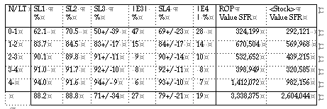
All simulations were run over the same subset of items and the same period of one year, all reorder points were calculated under an a-priori desired service level of P = 95 % requirement. The results were analysed by grouping the items by their average number of requests in the lead time N/LT.

If a method is successful, the desired service level P = 95 % will result in an observed service level distribution having an average P = 95 % and a small deviation. A large deviation can be interpreted as not successful. A deviation of almost zero, however is very unlikely to occur, there is an expected theoretical minimum for the deviation, which is reached if everything is optimal.

If the probability of each single request on being served is assumed to be equal to the desired service level P = 95 %, then for a lim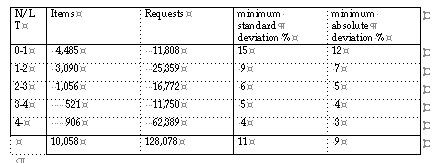ited number of serving events, for a particular item, the probability, mean and standard deviation of being served is given by the Bernoulli distribution.

e.g. x successful served on n serving events: P(x) = n!/( x! (n-x)! ) 0.95 ^x 0.05 ^n-x

The standard deviation can be calculated for each item, and the average value for each item group, denoted as minimum standard deviation is displayed together with the minimum absolute deviation in the GENERAL table.

The smallest spread around the desired value will outline the best procedure, however a smaller spread than the statistical minimum, is highly unlikely.

GENERAL P = 95 %

Single Demand method [3] based R

MAD based R

PERIODS based R

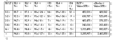
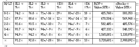
RESULTS CERN 95

CERN, the European Organisation for Nuclear Research, has been replacing its old logistic computer system, by a new computer system, a combination of the system TRITON handling the stores operations, and the system LOGIC calculating the logistic parameters. The transition of the old logistic system to the new system was effected in May 1995. The LOGIC parameters are based on the single demand distribution method [3]. Before the transition, optimisation was achieved by simulation and use of the optimisation modeling techniques of LOGIC. The task was not an easy one since "the science of extremes asks for the logistics of the extremes": long and variable lead times for specialistic items, which are ordered from the member states, in combination with the very variable demand patterns of the scientific demand, make the materials management a special demanding task.

Two important criteria to judge the performance of replenishment: the service levels (definition SL1 ) in combination with the stock values are represented below.

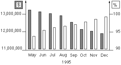
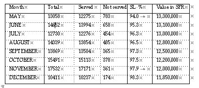
The CERN demand is scientific, non-commercial, low frequency type. More then 50 % of the items have a so-called lumpy, or erratic consumption pattern. The individual demanded quantities have often very broad requested quantity/single demand patterns. e.g. it is equally likely that someone asks for 5 m of a particular cable, as 5000 m of the same specific cable.

That the high service level is not a result of higher safety stocks, or changed lead times, or lower exception threshold level (which will cause more direct outs, can be concluded from the table below.

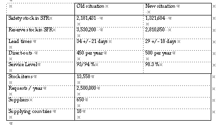
Safety stock Safety stock or buffer stock is the component of the reorder point aimed to set the level of item availability, or service level of the inventory by controlling the probability of stockout occurring.

Reserve stock Reserve stock or regular stock is the component of the reorder point R meeting the average demand in the average lead time.

Direct-outs Requests for exceptional quantities handled by special orders. The number shown does only include items which are normally served from stock, but excludes items which by policy, always are handled by direct-out.

Stock items Items which are normally served from stock. The total number of items handled is 15,037,and includes items which are normally served by EDI or by purchase order.

References

[1] R. E. Barlow, F. Proschan, Mathematical Theory of Reliability, John Wiley & Sons, Inc., New York, London, Sidney, 1967

[2] R. H. Ballou, Business Logistics Management, Prentice Hall Inc., 1992

[3] M. Krever, LOGIC/LIMS (Logistics Inventory Management System), CERN, 1996

[4] R. Dekker, H. Frenk, M. Kleijn, N. Piersma and T. de Kok, Report 9548/A; On the use of break quantities in multi-echelon distribution systems. Erasmus University Rotterdam, The Netherlands

[5] E. A. Silver, R. Peterson, Decision systems for inventory management and production planning, John Wiley & Sons, Inc., New York, London, Sidney, 1979. 1985

[6] M. Abramowitz and I. A. Stegun, Handbook of Mathematical Functions, Dover publications, Inc., New York, 1970